Do learning paradigms in context-aware Earth embeddings suppress spatial variability?
Geospatial embeddings (GE) offer user-friendly representations of large EO image archives with competitive performance across numerous predictive mapping applications. A wealth of GE are available, including Alpha Earth Foundations, TESSERA, or Major TOM.
Importantly, architectures behind GE differ fundamentally - we can discriminate pixel-level against context-aware architectures: embeddings based on one-dimensional architectures such as 1D CNNs or Transformers exploit the spectral, temporal, or spectral-temporal information contained in imagery archives at the pixel-level. Alternatively, context-aware embeddings based on CNNs, or Vision Transformers additionally learn not only the spectral and/or temporal signal contained in EO data but also the spatial context from neighboring pixels.
Context-awareness enables models to learn local spatial patterns such as texture, shape, or object extent, or in some cases even landscape-level patterns and structure that are characteristic of common targets in EO applications (e.g. land cover). The outputs of context-aware models tend to be more spatially coherent and robust to noise and local variability, improving thematic consistency at the patch or object scale.
Blurry Vision?
Alpha Earth Foundations (AEF) are currently one of the most prominent examples of context-aware embeddings and increasingly popular due to global and multi-year availability. AEF have been suggested to offer competitive performance for real-world downstream applications, including applications in agriculture, ecology, or land change science.
Context-aware embeddings tend to produce spatially coherent outputs, but we observed that predictions based on AEF tend to smooth high spatial variability in continuous targets compared to hand-crafted features from EO time series that represent exclusively information at the pixel-level. We then wondered if AEF inherently struggles to represent pronounced spatial variability in continuous targets but instead create smoothly appearing surfaces, precisely because of the context-aware learning paradigm. In other words - are we facing blurry vision when using AEF in applications targeting such high-variance contexts?

To be more precise, this observation was notably present when assessing predictions of fractional woody cover or canopy height in highly heterogeneous Miombo ecosystems, where dense vegetation canopies exist next to more open vegetation forms, but also isolated trees in larger patches of herbaceous vegetation. We observed a smoothness that partly resembled resampling issues, so we started to revisit the methods workflow but the issue persisted.
One potential reason behind this effect may be that AEF optimizes the reconstruction of spatially coherent or smooth targets such as climate, elevation, or land cover. Additionally, these tasks are being conducted in regions with rather homogeneous landscapes (i.e. low pixel-to-pixel variance) such as the US. Thus, during learning, the current AEF learning paradigm may favor consistent patches or smooth gradients, while the model is not rewarded to learn small-scale spatial semantics. Because of the target selection, the model succeeds at its objective without capturing fine spatial details contained in other contexts. This may systematically interfere with the learning of spatially variant and heterogeneous landscape contexts.
We want to explore this issue as a potential limitation of AEF in specific downstream applications where spatial variability is highly relevant, such as canopy height or biomass estimation.
Hypothesis
Current learning paradigms in spatially context-aware embeddings, such as AlphaEarth v1, dampen spatial variability in high-variance contexts, e.g. canopy height estimation.
Research Questions
- RQ 1: Which shallow ML model setup performs best for canopy height (CH) estimation?
- RQ 2: How does CH estimation performance differ between hand-crafted features (optical + radar STM), pixel-level (TESSERA) and context-aware (AEF) geospatial embeddings?
- RQ 3: How accurately is actual spatial variability in canopy height represented in predictions based on pixel-level vs. context-aware features?
Experiment
Study region
We explore canopy height estimation in Miombo woodlands in and around Gilé National Park, Mozambique. This is a heterogeneous, often open woody landscape with smallholder farmers relying on shifting cultivation, and regular fire occurrence.
Reference data
We use an aerial LiDAR Canopy Height Model at 1m resolution for the year 2022 by Demol et al. 2024, aggregated to 10 m using mean resampling.
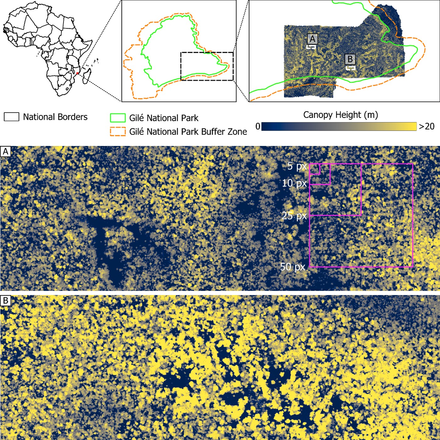
Study area and 1 m canopy height model used here. For reference, aggregation windows of 5, 10, 25, and 50 Sentinel-2 pixels are visualized
Input features
STM: As hand-crafted input features, we use bi-seasonal spectral-temporal metrics (STM) from Sentinel-1 and Sentinel-2 time series, comprising a total of 264 features per pixel.
AEF: Regarding context-aware GE we consider Alpha Earth Foundations (AEF) v1, which condense Sentinel-1, Sentinel-2 and Landsat time series into a 64-dimensional vector.
TESSERA: TESSERA v1.1 embeddings were selected as pixel-level GE, based on Sentinel-2 and Sentinel-1 time series which are represented as a 128-dimensional vector.
Workflow
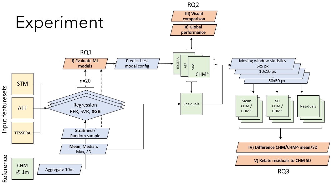
Experimental setup
We produced a stratified random sample (bins of 5m canopy height intervals with 1,000 samples in each bin) on the 10m aggregated mean canopy height layer and extracted the different input features for each sample. To evaluate the suitability of shallow ML models, we trained Random Forest Regressions, Support Vector Regressions, and XGBoost models with a 20-fold permutation varying the train / test split (70%/30%), predicted canopy height for the test samples, and evaluated the distribution of performance scores. Model evaluation was based on RMSE, MAE, ME, as well as R², intercept and slope of a linear model between observed and predicted canopy height.
We then produced spatial predictions to compare spatial patterns and variance between predictions. Comparison of global performance metrics (RMSE, MAE, R², etc.) was conducted across input features (STM, AEF, TESSERA) and models (XGBoost (XGB), Support Vector Regression (SVR), Random Forest Regression (RFR)). We deliberately chose to rely on shallow pixel-based ML algorithms for the canopy height predictions and did not test spatially aware CNNs to not conflate the spatial detail in the high-variance setting. This is potentially a self-imposed restriction on maximum attainable performance in this case but many users of GE oftentimes will rely on such shallow ML models.
Local spatial variance metrics were quantified by calculating mean, median, range, and standard deviation of canopy height between STM, AEF, TESSERA and reference (CHM) across non-overlapping windows of varying sizes (5x5, 10x10, 25x25 pixels) and comparing their statistical distributions. This was done to assess whether STMs, AEF, and TESSERA have varying distributions in terms of local spatial variance and to what extent it differs from the observed spatial variance. We then conclude the experiment by relating the observed performance to bins of spatial variance, investigating the question whether performance differences across the different input features are related to spatial variance.
Results
RQ1 - Model selection
We observe that AEF performs best throughout most of the experiments, with low error metrics and high R², followed by hand-crafted STM. TESSERA performed worst in our canopy height estimation setting.
While algorithm selection is not as straightforward and different algorithms show varying strengths depending on metrics and input features, we observed that XGBoost yielded a comparatively stable behaviour with high performance throughout and fits between observed and predicted that were close to the 1:1 line (i.e., intercepts close to 0, slopes close to 1). We thus continue the experiment using XGBoost. Overall, we want to note that the performance also depended on the sampling scheme chosen, but the overall patterns remained constant when altering between stratified vs. random sampling.
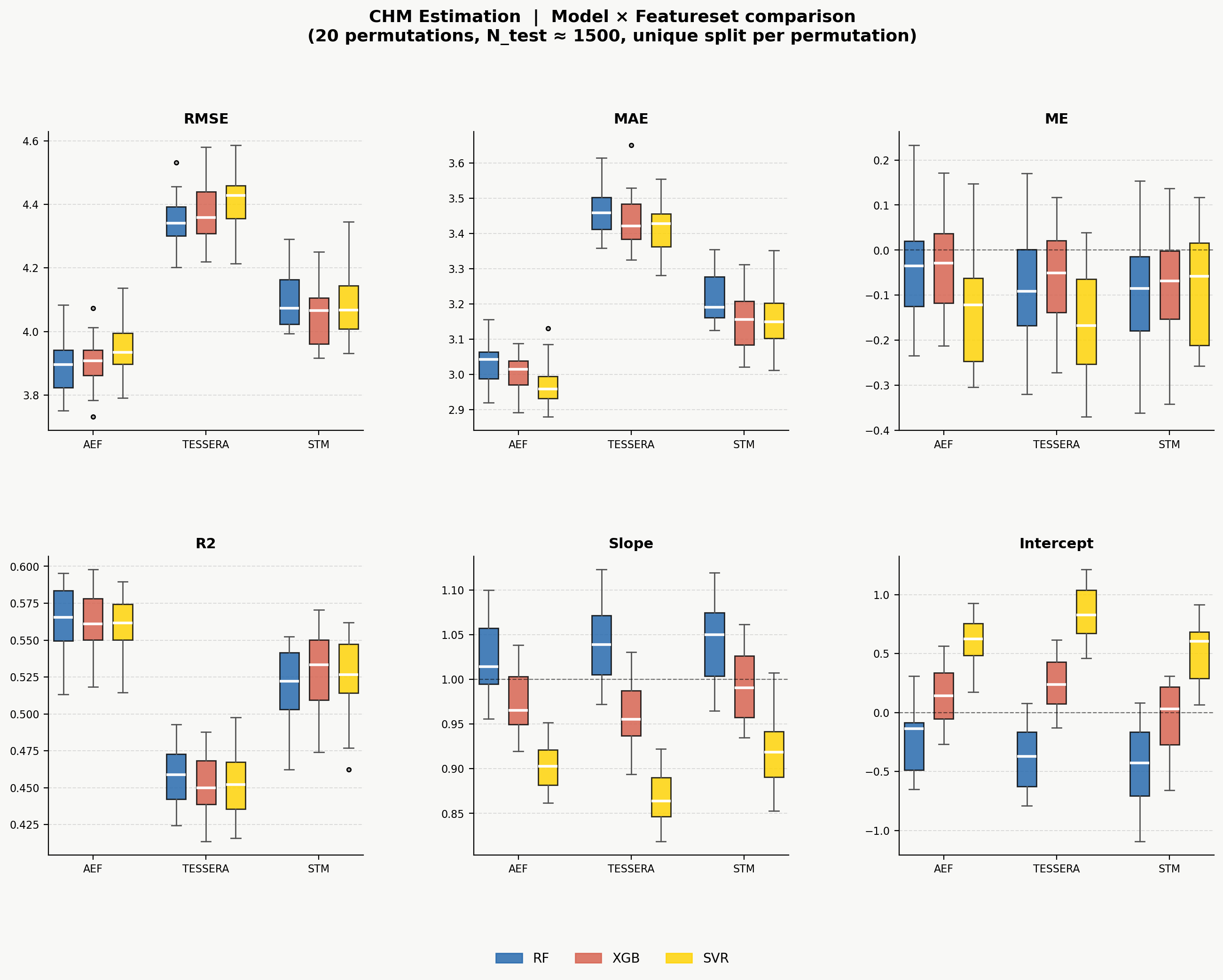
Canopy height estimation performance with different input features across model types and performance metrics. 20-fold permutations using different training / validation splits
RQ2 - Global performance
Global performance in the XGBoost setting indicates differences in performance between AEF & STM, whereas AEF consistently yields higher R² and lower RMSE and MAE compared to STM. The differences are partly marginal, while TESSERA had higher spread & stronger tendency for overestimation as observed in the scatterplots.
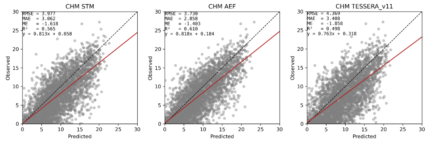
Scatterplots of observed vs. predicted (XGBoost) canopy height across input features.
RQ3 - Spatial variance
The spatial appearance of the canopy height predictions is quite distinct across the input features. As observed previously, AEF appears to have more smooth, continuous surfaces, with underestimation particularly in herbaceous wetland pockets that feature few large trees. Comparably, STM has visually higher pixel-level variability but also tendencies to overestimate canopy height in low woody cover regimes. TESSERA spatial patterns appear to be noisy with block-like artifacts.
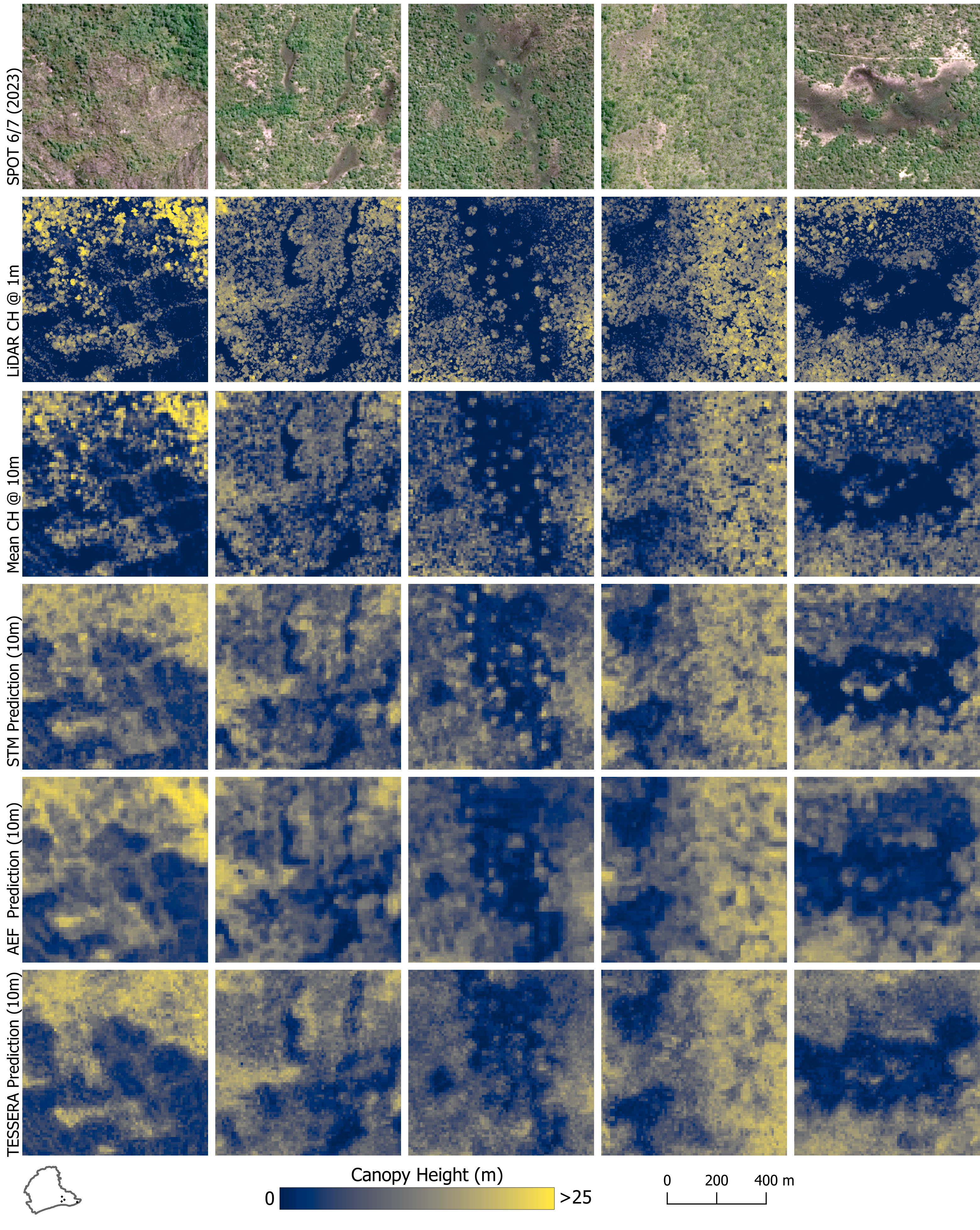
SPOT 6/7 1.5 m resolution imagery (first row), observed canopy height (second row) and predicted canopy height (third to last row) using XGBoost and STM, AEF, and TESSERA as input features.
Quantifying spatial variance
When quantifying the differences between reference and predicted canopy height mean or standard deviation in non-overlapping NxN pixel windows, more clear patterns emerge.
Overall, mean canopy height is consistently overestimated, whereas STM & AEF behave relatively similar, but TESSERA has a large spread.
The spatial variance (expressed as standard deviation in canopy height) is consistently underestimated across all sets of input features. Here, STM appears slightly closer to the 0 line, indicating that variance is picked up more consistently. But the question remains if the higher variance in STM predictions is actual (true) variance or simply noise resembling true variance?
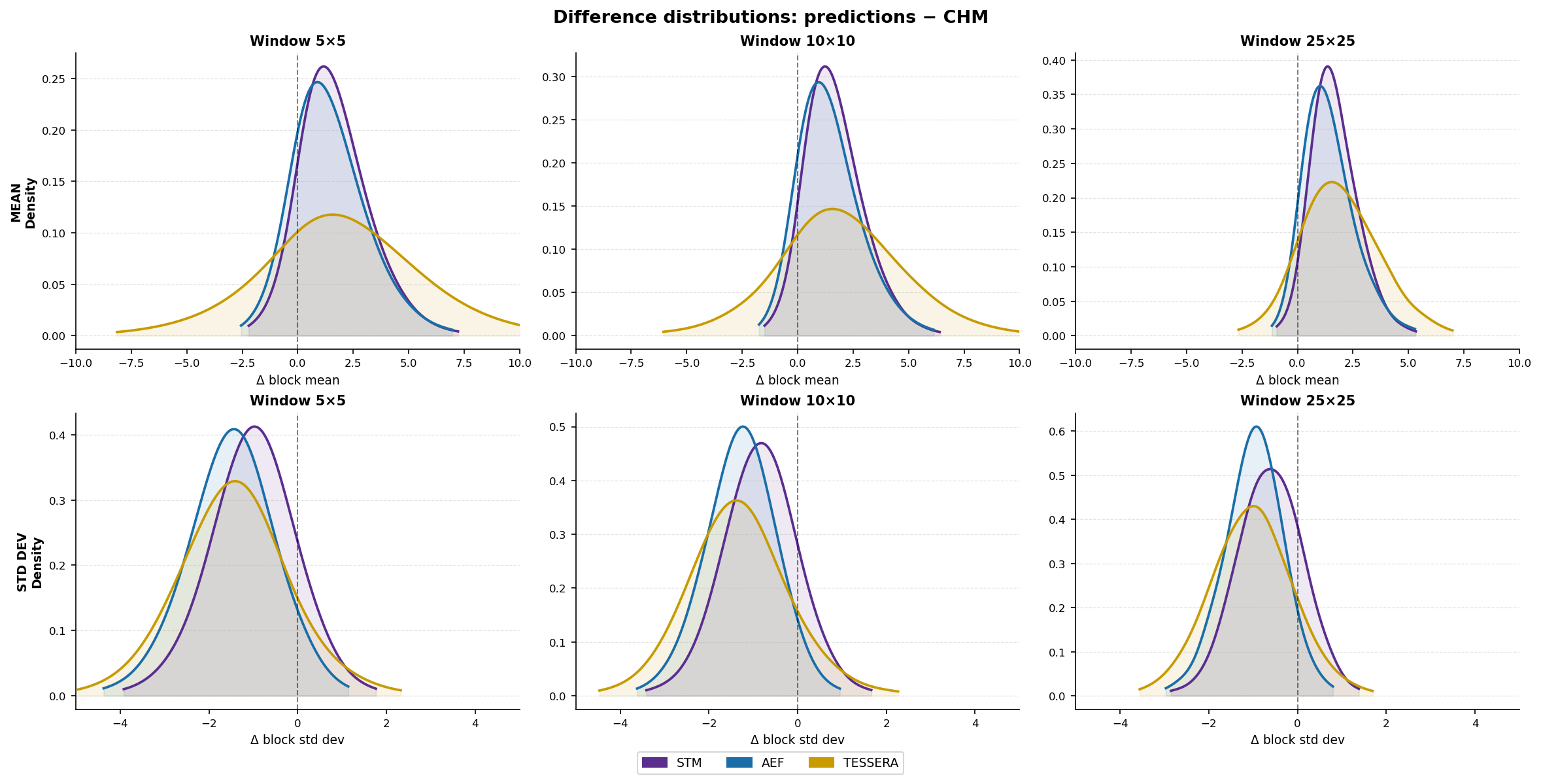
Density curves of difference in canopy height metrics (mean, standard deviation) between reference CHM and predictions across window sizes of 5, 10, and 25. Colors indicate input datasets used for predictions (STM, AEF, TESSERA).
Performance ~ Variance
To isolate the effect of artificial “blurriness” in high-variance settings, we related the observed variance (SD of canopy height representing spatial variability) to error metrics across the different N x N pixel windows. Following our hypothesis and empirical insights until this point we would expect that for AEF, errors increase with increasing spatial variance, while for TESSERA and STM this relationship should be less strong.
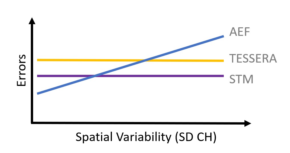
Schematic graph of hypothesis indicating decreasing performance with increasing spatial variance for AEF while STM and TESSERA remain constant performance.
Median trend lines for RMSE error metric indicate that this pattern is indeed present, although errors tend to increase across all input features and the differences between features are not very high. Nevertheless, we can show that compared to STM, AEF has lower errors in low-variance settings and higher errors in high-variance settings, partly confirming our initial hypothesis. This pattern holds true across window sizes but tends to average out when window sizes increase beyond 25 pixels. Similarly, it holds across RMSE, MAE, and ME. Nevertheless, we want to stress that the signal remains relatively weak, and differences are likely not statistically significant.
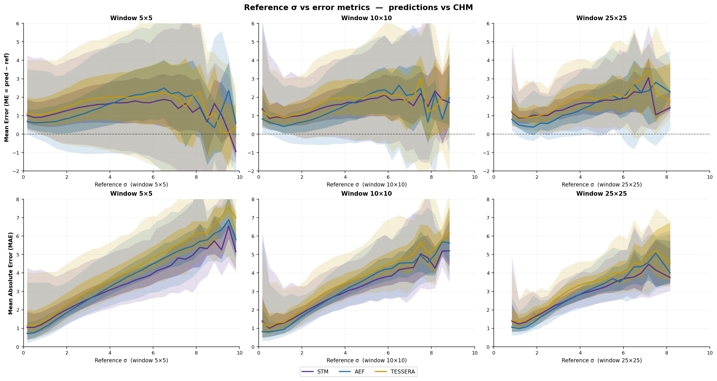
Median trends of ME and RMSE per bin of standard deviation in reference canopy height for 5x5, 10x10, and 25x25 pixel windows. Colors indicate different input features used.
Takeaways
The experiment yielded four takeaways which motivate further research:
Performance is sensitive to numerous design choices The performance of using GE in default workflows remains sensitive to methodological choices and these vary with input features. While trying to minimize these, the parameter space for adjusting the canopy height estimation workflow is still large with respect to, e.g. model choice, hyperparameters, the sampling scheme for selecting training and test data (purely random vs. stratified, and in the case of stratified sampling also the number and size of bins), and additional application-specific parameters such as the selection of the most appropriate canopy height metrics (i.e., mean vs. median vs. max at the 10m level).
Spatial patterns, consistency, and texture matter Isolating and quantifying visual effects and artefacts in GE and downstream predictions should be addressed more routinely. Qualitative inspection of input features may a valuable pointer towards issues related to input datasets, or as in this case, towards notions that may be embedded in model architectures or experimental setups. The problem at hand appears to be complex and distilling a measure of the desired effect (e.g., blurriness) is challenging, but further research could aim at testing more diverse measures of spatial autocorrelation, or advanced image processing metrics.
“Blurriness” is potentially embedded in learning paradigms Given the complexity of the AEF architecture, we can merely assume the reason for the effect of blurriness. First, smooth continuous training targets and regional bias as mentioned above may not lead to strong activation of the Precision block in comparison to the Space and Time blocks. Second, the AEF architecture features an initial spatial downsampling step (Figure 2 in the paper) decreasing the spatial resolution of the inputs by half before passing the inputs to the Space Time Precision encoder, which enhances computational efficiency but may contribute to the observed blurriness. Third, the STP encoder blends CNN (Precision) and attention blocks (Space, Time), the latter of which is running with coarser patch dimensions compared to the CNN (Precision) block. Fourth, reduced loss weights for some targets with coarse resolution such as GRACE Mass Grids (Table S2) could be interpreted as a consequence of smoothing effects of such predictors.
Pixel-level GE face different challenges Contrary to our expectations motivated by the literature, we were surprised that pixel-level GE such as TESSERA did not yield similar or higher performance compared to AEF and STM. This also involves the question of dimensionality, as TESSERA has a more nuanced representation with 128 dimensions as compared to the 64 dimensions of AEF. However, the spatial patterns in the TESSERA predictions indicate that there may be issues related to the pixel-level GE in our study region, which needs further investigation. We note, however, that the lack of spatial context embedded in TESSERA represents a competitive disadvantage which may be overcome by using context-sensitive, e.g. CNN-based, architectures for predicitons.
Contributors
This post was developed jointly with the DL4EO Special Interest Group with inputs from Jan Hemmerling, Leon-Friedrich Thomas and Pauline Hammer. We are grateful for valuable inputs from TESSERA author Madeline Lisaius (University of Cambridge) as well as members of the EOLab of Humboldt-Universität zu Berlin. We gratefully acknowledge access to the canopy height data granted by Miro Demol and Sylvera Ltd.
We would be interested in learning about your thoughts on this topic, so please feel free to reach out!